Table of Contents
This chapter describes data types and schema objects defined in the SQL standard.
Tibero provides various data types based on the SQL standard.
The Tibero data types are as follows:
| Classification | Data Type |
|---|---|
| String type | CHAR, VARCHAR, VARCHAR2, NCHAR, NVARCHAR, NVARCHAR2, RAW, LONG, LONG RAW |
| Number type | NUMBER, INTEGER, FLOAT, BINARY_FLOAT, BINARY_DOUBLE |
| Datetime type | DATE, TIME, TIMESTAMP, TIMESTAMP WITH TIME ZONE, TIMESTAMP WITH LOCAL TIME ZONE |
| Interval type | INTERVAL YEAR TO MONTH, INTERVAL DAY TO SECOND |
| Large object type | CLOB, BLOB, XMLTYPE |
| Embedded type | ROWID |
| User-defined type | ARRAY, NESTED TABLE |
String types store strings. CHAR, VARCHAR, VARCHAR2, NCHAR, NVARCHAR, NVARCHAR2, RAW, LONG, and LONG RAW types are classified as string types.
CHAR
The CHAR type stores fixed-length character strings.
CHAR(size[BYTE|CHAR])
The CHAR type has the following characteristics:
-
This type can be declared with a size of up to 2,000 bytes.
If a converted string exceeds 2,000 bytes, an error will occur.
Tibero converts strings entered in a CHAR column to strings appropriate for the database character set before storing them. The converted strings must not exceed 2,000 bytes.
-
Strings are stored as bytes or characters.
Strings are declared as the following format: CHAR (10, BYTE) or CHAR (10, CHAR). If the second parameter is not specified like CHAR (10), strings are stored in bytes by default.
When declaring each string as an array of bytes, up to 2000 bytes can be stored. When declaring as CHAR, up to 2000 characters can be stored. If strings are stored as characters, the length of a column depends on the character set used by a database because the size (in bytes) of a character can differ.
-
When using CHAR type data in SQL statements, make sure to use single quotes (' ').
-
If a string length is 0, the data is treated as NULL.
The following example illustrates the use of the CHAR type:
PRODUCT_NAME
      CHAR(10)
In the above example, the PRODUCT_NAME column contains 10-byte character strings. If the length of an entered string is shorter than the declared type, the remainder will be blank-padded. For example, if 'Tibero' is entered, four blank spaces will be padded and 'Tibero____' will be stored.
VARCHAR
The VARCHAR type stores variable-length character strings.
VARCHAR(size[BYTE|CHAR])
The VARCHAR type has the following characteristics:
-
This type can be declared with a size of up to 65,532 bytes.
If a converted string exceeds 65,532 bytes, an error will occur.
Tibero converts strings entered in a VARCHAR column to strings appropriate for the database character set before storing them. The converted strings must not exceed 65,532 bytes.
-
Strings are stored as bytes or characters.
Strings are declared using the following format: VARCHAR (10, BYTE) or VARCHAR (10, CHAR). If the second parameter is not specified, as in VARCHAR (10), strings are stored as bytes.
When declaring each string as an array of bytes, up to 65,532 bytes can be stored. When declaring as CHAR, up to 65,532 characters can be stored. If strings are stored as characters, the length of a column depends on the character set used by a database because the size (in bytes) of a character can differ.
-
When using VARCHAR type data in SQL statements, make sure to use single quotes (' ').
-
If a string length is 0, the data is treated as NULL.
The following example illustrates the use of the VARCHAR type:
EMP_NAME
      VARCHAR(10)
In the above example, the EMP_NAME column has 10-byte character strings. For example, if 'Peter' is entered, 'Peter' will be stored without any change. Therefore, the actual stored string length is 5 bytes while the EMP_NAME column is declared as 10 bytes.
Like this, the VARCHAR type has variable-length strings up to a maximum of the declared length.
VARCHAR2
The VARCHAR2 type is exactly the same as the VARCHAR type.
NCHAR
The NCHAR type stores fixed-length Unicode character strings.
NCHAR(size)
The NCHAR type has the following characteristics:
-
This type is similar to the CHAR type, but strings are always stored in characters.
The length of a column depends on the international character set used by the database. For example, the maximum length of a column in UTF8 or UTF16 can triple or double, respectively.
-
The NCHAR type can be declared with a size of up to 65,532 characters.
-
When using NCHAR type data in SQL statements, make sure to use single quotes (' ').
-
If a string length is 0, the data is treated as NULL.
NVARCHAR
The NVARCHAR type stores variable-length Unicode character strings.
NVARCHAR(size)
The NVARCHAR type has the following characteristics:
-
This type is similar to the VARCHAR type, but strings are always stored in characters.
The length of a column depends on the international character set used by the database. For example, the maximum length of a column in UTF8 or UTF16 can triple or double, respectively.
-
The NVARCHAR type can be declared with a size of up to 4,000 characters.
-
When using NVARCHAR type data in SQL statements, make sure to use single quotes (' ').
-
If a string length is 0, the data is treated as NULL.
NVARCHAR2
The NVARCHAR2 type is the same as the NVARCHAR type.
RAW
The RAW type stores variable-length binary data.
The RAW type can have NULL characters ('\0') in the middle of a string unlike the CHAR and VARCHAR types. This type always stores length information because a NULL character cannot indicate the end of the data.
RAW(size)
The RAW type has the following characteristics:
-
This type can be declared with a size of up to 2,000 bytes.
-
Variable-length binary data within a declared length is stored.
-
NULL characters ('\0') can be located in the middle of a string.
-
When input/output tasks are performed, data is expressed in hexadecimal format.
For example, 4 bytes of data is expressed as '012345AB' in hexadecimal format. If necessary, data can start with 0.
LONG
The LONG type is an expanded version of the VARCHAR type. This type stores character strings in the same way as the VARCHAR type.
LONG
The LONG type has the following characteristics:
-
This type can be declared with a size of up to 2 gigabytes.
-
Only one column in a table can be declared as this type.
-
An index cannot be created for this type of column.
-
When a row that includes this type of data is stored, the data is stored in the same disk block with other column data. The data may be stored in several disk blocks depending on its length.
-
This type of data can only be accessed serially. Performing an operation at an arbitrary location is not possible.
LONG
      RAW
The LONG RAW type is an expanded version of the RAW type. This type stores binary data in the same way as the RAW type.
LONG
RAW
The LONG RAW type has the following characteristics:
-
This type can be declared with a size of up to 2 gigabytes.
-
Only one column in a table can be declared as this type.
-
An index cannot be created for this type of column.
-
When a row that includes this type of data is stored, the data is stored in the same disk block with other column data. The data may be stored in several disk blocks according to its length.
-
This type of data can only be accessed serially. Performing an operation at an arbitrary location is impossible.
Number types store integers and real numbers. NUMBER, INTEGER, FLOAT, and BINARY_DOUBLE types are classified as number types.
Tibero supports the SQL standard number types specified in ANSI. Therefore, when a column is declared as INTEGER or FLOAT, the column type is changed to the NUMBER type after precision and scale are set internally.
Note
In this document, the INTEGER and FLOAT types are not described.
NUMBER
The NUMBER type stores integers and real numbers.
The NUMBER type stores a number of up to 38 digits. The absolute value is between 1.0×10-130 and 1.0×10126. It can also store the values of positive infinity, negative infinity, and zero.
The NUMBER type can be declared with precision and scale.
NUMBER[(precision[,scale])]
| Option | Description |
|---|---|
| Precision | If set to an asterisk, arbitrary number of digits less than 39 can be stored. In general, scale is set together. |
| Scale | The number of digits to the right of the decimal point.
|
If NUMBER data is declared without precision and scale, all data are supported within the maximum range and precision. Data with a precision greater than 38 is rounded.
The following table shows how input data would be stored based on the precision and the scale values.
| Input Data | NUMBER Type Declaration | Actual Stored Data |
|---|---|---|
| 12,345.678 | NUMBER | 12,345.678 |
| 12,345.678 | NUMBER(*,3) | 12,345.678 |
| 12,345.678 | NUMBER(8,3) | 12,345.678 |
| 12,345.678 | NUMBER(8,2) | 12,345.68 |
| 12,345.678 | NUMBER(8) | 12,346 |
| 12,345.678 | NUMBER(8,-2) | 12,300 |
| 12,345.678 | NUMBER(3) | Cannot be stored because the total number of digits of input data exceeds the set precision. |
BINARY_FLOAT
The BINARY_FLOAT type stores real numbers and integers. It is a single-precision 32-bit floating point data type.
A BINARY_FLOAT variable can be set to positive infinity, negative infinity, and zero. The absolute value range is 1.17549E-38 to 3.40282E+38.
The BINARY_FLOAT type has the following characteristics:
-
Supports special values such as INF, -INF, and NaN (Not A Number).
-
Supports the four fundamental arithmetic operations.
-
Supports the comparison operator. However, in Tibero, NaN is greater than any numeric value, and different NaN values are considered equal.
-
Supports a variety of conversion functions and mathematical functions.
BINARY_DOUBLE
The BINARY_DOUBLE typestores real numbers and integers. It is a double-precision 64-bit floating point data type.
A BINARY_DOUBLE variable can be set to positive infinity, negative infinity, and zero. The absolute value range is 1.79769313486231E+308 to 2.22507485850720E-308.
The BINARY_DOUBLE type has the following characteristics:
-
Supports special values such as INF, -INF, and NaN (Not A Number).
-
Supports the four fundamental arithmetic operations.
-
Supports the comparison operator. However, in Tibero, NaN is greater than any numeric value, and different NaN values are considered equal.
-
Supports a variety of conversion functions and mathematical functions.
Priority of NUMBER TYPE
Tibero converts numbers to different data types according to the priority. The order of priority from highest to lowest: BINARY_DOUBLE, BINARY_FLOAT, then NUMBER.
-
Converts all operators to BINARY_DOUBLE if even a single operator is BINARY_DOUBLE.
-
Converts all operators to BINARY_FLOAT if no BINARY_DOUBLE operators are used and at least a single operator is BINARY_FLOAT.
-
Converts all operators to NUMBER when there are no BINARY_FLOAT or BINARY_DOUBLE operators.
BINARY_DOUBLE, BINARY_FLOAT, and NUMBER have lower priority than the datetime or interval types, but they have higher priority than other types.
Datetime types store times and dates. DATE, TIME, TIMESTAMP, TIMESTAMP WITH TIME ZONE, and TIMESTAMP WITH LOCAL TIME ZONE types are classified as datetime types.
DATE
The DATE type stores specific times ranging from seconds to years.
DATE
The DATE type has the following characteristics:
-
Years, months, days, hours, minutes, and seconds can be stored.
-
Years can be a number between BC 9,999 and AD 9,999.
-
Hours are expressed in the 24-hour format.
TIME
The TIME type stores specific times in seconds with up to nine decimal places.
TIME
      [(fractional_seconds_precision)]
| Item | Description |
|---|---|
| fractional_seconds_precision | Number of decimal places to store. A number from 0 to 9 can be specified (Default value: 6) |
The TIME type has the following characteristics:
-
Hours, minutes, seconds, and nanoseconds can be stored.
-
Hours are expressed in the 24-hour format.
TIMESTAMP
The TIMESTAMP type stores specific dates and times in seconds down to nine decimal places.
TIMESTAMP
      [(fractional_seconds_precision)]
| Item | Description |
|---|---|
| fractional_seconds_precision | Number of decimal places to store. A number from 0 to 9 can be specified. (Default value: 6) |
The TIMESTAMP type has the following characteristics:
-
Years, months, days, hours, minutes, seconds, and nanoseconds can be stored.
-
Years can be a number between BC 9,999 and AD 9,999.
-
Hours are expressed in the 24-hour format.
TIMESTAMP WITH TIME ZONE
The TIMESTAMP WITH TIME ZONE type stores specific time zones as well as dates and times.
TIMESTAMP
      [(fractional_seconds_precision)] WITH TIME ZONE
| Item | Description |
|---|---|
| fractional_seconds_precision | Number of decimal places to store. A number from 0 to 9 can be specified (Default value: 6) |
The TIMESTAMP WITH TIME ZONE type has the following characteristics:
-
Like the TIMESTAMP type, years, months, days, hours, minutes, seconds, and nanoseconds can be stored.
-
The values described above are normalized to UTC (Coordinated Universal Time).
-
A time zone displayed as a local name or an offset is also stored. The offset represents the difference between the local time and the UTC time.
TIMESTAMP WITH LOCAL TIME ZONE
The TIMESTAMP WITH LOCAL TIME ZONE type stores different times depending on the time zone of a particular session.
TIMESTAMP
      [(fractional_seconds_precision)] WITH LOCAL TIME ZONE
| Item | Description |
|---|---|
| fractional_seconds_precision | Number of decimal places to store. A number from 0 to 9 can be specified (Default value: 6) |
The TIMESTAMP WITH LOCAL TIME ZONE type has the following characteristics:
-
Like the TIMESTAMP type, years, months, days, hours, minutes, seconds, and nanoseconds can be stored.
-
The values described above are normalized to UTC (Coordinated Universal Time).
-
Unlike the TIMESTAMP WITH TIME ZONE type, the TIMESTAMP WITH LOCAL TIME ZONE type does not store local names or offsets, but automatically modifies the time zone to that of the session with which the user searches.
Interval types store a difference between times or dates. INTERVAL YEAR TO MONTH and INTERVAL DAY TO SECOND types are classified as interval types.
INTERVAL YEAR TO MONTH
The INTERVAL YEAR TO MONTH type stores time intervals with years and months.
INTERVAL YEAR
      [(year_precision)] TO MONTH
| Item | Description |
|---|---|
| year_precision | Number of digits of a year value. (Default value: 2) |
INTERVAL DAY TO SECOND
The INTERVAL DAY TO SECOND type stores time intervals with days, hours, minutes, and seconds.
INTERVAL DAY
      [(day_precision)] TO SECOND
      [(fractional_seconds_precision)]
| Item | Description |
|---|---|
| day_precision | Number of digits of a day value. (Default value: 2) |
| fractional_seconds_precision | Number of decimal places to store. A number from 0 to 9 can be specified. (Default value: 6) |
Large object types store large objects. CLOB, BLOB, and XMLTYPE types are classified as large object types.
CLOB
The CLOB type is an expanded version of the LONG type.
The CLOB type has the following characteristics:
-
This type can be declared with a size of up to 4 gigabytes.
-
One or more columns in a table can be declared as this type.
-
Unlike the LONG type, accessing an arbitrary location is possible.
-
Data in this type of column is not stored in the same disk block with data from other types of columns.
Rows in the disk block only have pointers to the CLOB data, which is stored in separate disk blocks.
BLOB
The BLOB type is an expanded version of the LONG RAW type.
The BLOB type has the following characteristics:
-
This type can be declared with a size of up to 4 gigabytes.
-
One or more columns in a table can be declared as this type.
-
Unlike the LONG RAW type, accessing an arbitrary location is possible.
-
Data in this type of column is not stored in the same disk block with data from other types of columns.
Rows in the disk block have only pointers to the BLOB data which is stored in separate disk blocks.
XMLTYPE
XML (Extensible Markup Language), a standard introduced by the W3C (World Wide Web Consortium), expresses any kind of data, regardless of structure. To store XML data, Tibero provides the XMLTYPE type that is internally stored as the CLOB type.
The XMLTYPE type has the following characteristics:
-
Data as large as the maximum size of CLOB can be stored.
-
One or more columns in a table can be declared as this type.
-
This type is used to access, extract, or inquire about XML data.
Embedded types are automatically inserted in every row by Tibero. The ROWID type is classified as an embedded type.
ROWID
The ROWID type is inserted in every row by Tibero to identify each row in a database. This type stores the physical location of each row.
ROWID
Note
For more information about ROWID, refer to “2.5. Pseudo Columns”.
A user-defined type can be used as a tbPSM type and can be stored in Tibero. User-defined types include arrays and nested tables. For more information, refer to Tibero tbPSM Guide.
Array
Array is a collection of data with the same type. The type and length of the array are defined by the user.
Note
For more information, refer to Tibero tbPSM Guide.
Nested Table
Nested table is a collection of data with the same type. The type is defined by the user, but there is no length.
Note
For more information, refer to Tibero tbPSM Guide.
This section describes how to convert data types for comparison, operation, etc. in Tibero.
Data type conversion can be performed explicitly by the user or implicitly.
The user can directly use SQL conversion functions to convert data types.
The following is a list of type conversion functions. (Rows are types before conversion, and columns are types after conversion)
[Table 2.1] Explicit Type Conversion (1)
| from \ to | CHAR, VARCHAR2, NCHAR, NVARCHAR2 | NUMBER | Date, Time and Interval |
|---|---|---|---|
CHAR, VARCHAR2, NCHAR, NVARCHAR2 | TO_CHAR, TO_NCHAR | TO_NUMBER | TO_DATE, TO_TIME, TO_TIMESTAMP, TO_TIMESTAMP_TZ, TO_DSINTERVAL, TO_YMINTERVAL |
| NUMBER | TO_CHAR, TO_NCHAR | - | NUMTOYMINTERVAL, NUMTODSINTERVAL |
| Date, Time and Interval | TO_CHAR, TO_NCHAR | X | - |
| RAW | RAWTOHEX | X | X |
| ROWID | ROWIDTOCHAR | X | X |
LONG, LONG RAW | LONG_TO_CHAR | X | X |
CLOB, NCLOB, BLOB | TO_CHAR, TO_NCHAR | X | X |
| BINARY_FLOAT | TO_CHAR, TO_NCHAR | TO_NUMBER | X |
| BINARY_DOUBLE | TO_CHAR, TO_NCHAR | TO_NUMBER | X |
[Table 2.2] Explicit Type Conversion (2)
| from \ to | BINARY_DOUBLE | RAW | ROWID |
|---|---|---|---|
CHAR, VARCHAR2, NCHAR, NVARCHAR2 | TO_BINARY_DOUBLE | HEXTORAW | CHARTOROWID |
| NUMBER | TO_BINARY_DOUBLE | X | X |
Date, Time and Interval | X | X | X |
| RAW | - | - | X |
| ROWID | X | X | - |
LONG, LONG RAW | X | X | X |
CLOB, NCLOB, BLOB | X | X | X |
| BINARY_FLOAT | X | X | X |
| BINARY_DOUBLE | X | X | X |
[Table 2.3] Explicit Type Conversion (3)
| from \ to | LONG, LONG RAW | CLOB, NCLOB, BLOB | BINARY_FLOAT | BINARY_DOUBLE |
|---|---|---|---|---|
CHAR, VARCHAR2, NCHAR, NVARCHAR2 | LONG_TO_CHAR | TO_CLOB | TO_BINARY_FLOAT | TO_BINARY_DOUBLE |
| NUMBER | X | X | TO_BINARY_FLOAT | TO_BINARY_DOUBLE |
| Date, Time and Interval | X | X | X | X |
| RAW | X | TO_BLOB | X | X |
| ROWID | X | X | X | X |
LONG, LONG RAW | - | TO_LOB | X | X |
CLOB, NCLOB, BLOB | X | TO_CLOB | X | X |
| BINARY_FLOAT | X | X | TO_BINARY_FLOAT | TO_BINARY_DOUBLE |
| BINARY_DOUBLE | X | X | TO_BINARY_FLOAT | TO_BINARY_DOUBLE |
Implicit conversion is performed automatically as needed without user specifying explicit conversion.
Implicit type conversion is needed in the following cases:
-
When inserting or updating a column with a data type that is different from the column data type
-
When comparing different types in a conditional clause
The following is an implicit type conversion matrix. (Rows are types before conversion, and columns are types after conversion).
[Table 2.4] Implicit Type Conversion (1)
| NUMBER | CHAR | VARCHAR2 | RAW | DATE | TIME | TIMESTAMP | |
|---|---|---|---|---|---|---|---|
| NUMBER | - | O | O | X | X | X | X |
| CHAR | O | - | O | O | O | O | O |
| VARCHAR2 | O | O | - | O | O | O | O |
| RAW | X | O | O | - | X | X | X |
| DATE | X | O | O | X | - | X | O |
| TIME | X | O | O | X | X | - | X |
| TIMESTAMP | X | O | O | X | O | X | - |
| INTERVAL YEAR TO MONTH | X | O | O | X | X | X | X |
| INTERVAL DAY TO SECOND | X | O | O | X | X | X | X |
| LONG | X | X | X | X | X | X | X |
| LONG RAW | X | X | X | X | X | X | X |
| BLOB | X | X | X | O | X | X | X |
| CLOB | X | O | O | X | X | X | X |
| ROWID | X | O | O | X | X | X | X |
| NCHAR | O | O | O | O | O | O | O |
| NVARCHAR2 | O | O | O | O | O | O | O |
| NCLOB | X | O | O | X | X | X | X |
| TIMESTAMP WITH TIMEZONE | X | O | O | X | O | X | O |
| TIMESTAMP WITH LOCAL TIMEZONE | X | O | O | X | O | X | O |
| BINARY_FLOAT | O | O | O | X | X | X | X |
| BINARY_DOUBLE | O | O | O | X | X | X | X |
[Table 2.5] Implicit Type Conversion (2)
| INTERVAL YEAR TO MONTH | INTERVAL DAY TO SECOND | LONG | LONG RAW | BLOB | CLOB | ROWID | |
|---|---|---|---|---|---|---|---|
| NUMBER | X | X | O | X | X | O | X |
| CHAR | O | O | O | O | O | O | O |
| VARCHAR2 | O | O | O | O | O | O | O |
| RAW | X | X | O | O | O | O | X |
| DATE | X | X | O | X | X | X | X |
| TIME | X | X | O | X | X | X | X |
| TIMESTAMP | X | X | O | X | X | X | X |
| INTERVAL YEAR TO MONTH | - | X | O | X | X | X | X |
| INTERVAL DAY TO SECOND | X | - | O | X | X | X | X |
| LONG | X | X | - | X | X | X | X |
| LONG RAW | X | X | X | - | X | X | X |
| BLOB | X | X | X | O | - | X | X |
| CLOB | X | X | O | X | X | - | X |
| ROWID | X | X | O | X | X | X | - |
| NCHAR | O | O | O | O | X | O | O |
| NVARCHAR2 | O | O | O | O | X | O | O |
| NCLOB | X | X | O | X | X | O | X |
| TIMESTAMP WITH TIMEZONE | X | X | O | X | X | X | X |
| TIMESTAMP WITH LOCAL TIMEZONE | X | X | O | X | X | X | X |
| BINARY_FLOAT | X | X | O | X | X | X | X |
| BINARY_DOUBLE | X | X | O | X | X | X | X |
[Table 2.6] Implicit Type Conversion (3)
| NCHAR | NVARCHAR2 | NCLOB | TIMESTAMP WITH TIMEZONE | TIMESTAMP WITH LOCAL TIMEZONE | BINARY_FLOAT | BINARY_DOUBLE | |
|---|---|---|---|---|---|---|---|
| NUMBER | O | O | X | X | X | O | O |
| CHAR | O | O | O | O | O | O | O |
| VARCHAR2 | O | O | O | O | O | O | O |
| RAW | O | O | X | X | X | X | X |
| DATE | O | O | X | O | O | X | X |
| TIME | O | O | X | X | X | X | X |
| TIMESTAMP | O | O | X | O | O | X | X |
| INTERVAL YEAR TO MONTH | O | O | X | X | X | X | X |
| INTERVAL DAY TO SECOND | O | O | X | X | X | X | X |
| LONG | X | X | X | X | X | X | X |
| LONG RAW | X | X | X | X | X | X | X |
| BLOB | X | X | X | X | X | X | X |
| CLOB | O | O | O | X | X | X | X |
| ROWID | O | O | X | X | X | X | X |
| NCHAR | - | O | O | O | O | O | O |
| NVARCHAR2 | O | - | O | O | O | O | O |
| NCLOB | O | O | - | X | X | X | X |
| TIMESTAMP WITH TIMEZONE | O | O | X | - | O | X | X |
| TIMESTAMP WITH LOCAL TIMEZONE | O | O | X | O | - | X | X |
| BINARY_FLOAT | O | O | X | X | X | - | O |
| BINARY_DOUBLE | O | O | X | X | X | O | - |
Type Comparison
The following matrix shows the type with higher precedence when comparing two data types.
[Table 2.7] Type Comparison (1)
| NUMBER | CHAR | VARCHAR2 | RAW | |
|---|---|---|---|---|
| NUMBER | NUMBER | NUMBER | NUMBER | VARCHAR2 |
| CHAR | NUMBER | CHAR | VARCHAR2 | CHAR |
| VARCHAR2 | NUMBER | VARCHAR2 | VARCHAR2 | VARCHAR2 |
| RAW | VARCHAR2 | CHAR | VARCHAR2 | RAW |
| DATE | X | DATE | DATE | VARCHAR2 |
| TIME | X | TIME | TIME | VARCHAR2 |
| TIMESTAMP | VARCHAR2 | TIMESTAMP | TIMESTAMP | VARCHAR2 |
| INTERVAL YEAR TO MONTH | VARCHAR2 | INTERVAL YEAR TO MONTH | INTERVAL YEAR TO MONTH | VARCHAR2 |
| INTERVAL DAY TO SECOND | VARCHAR2 | INTERVAL DAY TO SECOND | INTERVAL DAY TO SECOND | VARCHAR2 |
| LONG | X | LONG | LONG | VARCHAR2 |
| LONG RAW | VARCHAR2 | LONG | LONG | VARCHAR2 |
| BLOB | X | X | X | X |
| CLOB | X | CLOB | CLOB | CLOB |
| ROWID | VARCHAR2 | ROWID | ROWID | VARCHAR2 |
| NCHAR | NUMBER | NCHAR | NVARCHAR2 | NCHAR |
| NVARCHAR2 | NUMBER | NVARCHAR2 | NVARCHAR2 | NVARCHAR2 |
| NCLOB | X | NCLOB | NCLOB | NCLOB |
| TIMESTAMP WITH TIMEZONE | VARCHAR2 | TIMESTAMP | TIMESTAMP | VARCHAR2 |
| TIMESTAMP WITH LOCAL TIMEZONE | VARCHAR2 | TIMESTAMP | TIMESTAMP | VARCHAR2 |
| BINARY_FLOAT | BINARY_FLOAT | BINARY_FLOAT | BINARY_FLOAT | VARCHAR2 |
| BINARY_DOUBLE | BINARY_DOUBLE | BINARY_DOUBLE | BINARY_DOUBLE | VARCHAR2 |
[Table 2.8] Type Comparison (2)
| DATE | TIME | TIMESTAMP | INTERVAL YEAR TO MONTH | |
|---|---|---|---|---|
| NUMBER | X | X | VARCHAR2 | VARCHAR2 |
| CHAR | DATE | TIME | TIMESTAMP | INTERVAL YEAR TO MONTH |
| VARCHAR2 | DATE | TIME | TIMESTAMP | INTERVAL YEAR TO MONTH |
| RAW | VARCHAR2 | VARCHAR2 | VARCHAR2 | VARCHAR2 |
| DATE | DATE | VARCHAR2 | TIMESTAMP | VARCHAR2 |
| TIME | VARCHAR2 | TIME | VARCHAR2 | VARCHAR2 |
| TIMESTAMP | TIMESTAMP | VARCHAR2 | TIMESTAMP | VARCHAR2 |
| INTERVAL YEAR TO MONTH | VARCHAR2 | VARCHAR2 | VARCHAR2 | INTERVAL YEAR TO MONTH |
| INTERVAL DAY TO SECOND | VARCHAR2 | VARCHAR2 | VARCHAR2 | INTERVAL DAY TO SECOND |
| LONG | X | X | X | X |
| LONG RAW | VARCHAR2 | VARCHAR2 | VARCHAR2 | VARCHAR2 |
| BLOB | X | X | X | X |
| CLOB | X | X | X | X |
| ROWID | VARCHAR2 | VARCHAR2 | VARCHAR2 | VARCHAR2 |
| NCHAR | DATE | TIME | TIMESTAMP | INTERVAL YEAR TO MONTH |
| NVARCHAR2 | DATE | TIME | TIMESTAMP | INTERVAL YEAR TO MONTH |
| NCLOB | X | X | X | X |
| TIMESTAMP WITH TIMEZONE | TIMESTAMP | VARCHAR2 | TIMESTAMP WITH TIMEZONE | VARCHAR2 |
| TIMESTAMP WITH LOCAL TIMEZONE | TIMESTAMP | VARCHAR2 | TIMESTAMP WITH LOCAL TIMEZONE | VARCHAR2 |
| BINARY_FLOAT | X | X | VARCHAR2 | VARCHAR2 |
| BINARY_DOUBLE | X | X | VARCHAR2 | VARCHAR2 |
[Table 2.9] Type Comparison (3)
| INTERVAL DAY TO SECOND | LONG | LONG RAW | BLOB | |
|---|---|---|---|---|
| NUMBER | VARCHAR2 | X | VARCHAR2 | X |
| CHAR | INTERVAL DAY TO SECOND | LONG | LONG | X |
| VARCHAR2 | INTERVAL DAY TO SECOND | LONG | LONG | X |
| RAW | VARCHAR2 | VARCHAR2 | VARCHAR2 | X |
| DATE | VARCHAR2 | X | VARCHAR2 | X |
| TIME | VARCHAR2 | X | VARCHAR2 | X |
| TIMESTAMP | VARCHAR2 | X | VARCHAR2 | X |
| INTERVAL YEAR TO MONTH | VARCHAR2 | X | VARCHAR2 | X |
| INTERVAL DAY TO SECOND | VARCHAR2 | X | VARCHAR2 | X |
| LONG | X | LONG | LONG | X |
| LONG RAW | VARCHAR2 | LONG | LONG RAW | X |
| BLOB | X | X | X | BLOB |
| CLOB | X | LONG | LONG | X |
| ROWID | VARCHAR2 | ROWID | VARCHAR2 | X |
| NCHAR | INTERVAL DAY TO SECOND | X | X | X |
| NVARCHAR2 | INTERVAL DAY TO SECOND | X | X | X |
| NCLOB | X | X | X | X |
| TIMESTAMP WITH TIMEZONE | VARCHAR2 | X | VARCHAR2 | X |
| TIMESTAMP WITH LOCAL TIMEZONE | VARCHAR2 | X | VARCHAR2 | X |
| BINARY_FLOAT | VARCHAR2 | X | VARCHAR2 | X |
| BINARY_DOUBLE | VARCHAR2 | X | VARCHAR2 | X |
[Table 2.10] Type Comparison (4)
| CLOB | ROWID | NCHAR | NVARCHAR2 | |
|---|---|---|---|---|
| NUMBER | X | VARCHAR2 | NUMBER | NUMBER |
| CHAR | CLOB | ROWID | NCHAR | NVARCHAR2 |
| VARCHAR2 | CLOB | ROWID | NCHAR | NVARCHAR2 |
| RAW | CLOB | VARCHAR2 | NCHAR | NVARCHAR2 |
| DATE | X | VARCHAR2 | DATE | DATE |
| TIME | X | VARCHAR2 | TIME | TIME |
| TIMESTAMP | X | VARCHAR2 | TIMESTAMP | TIMESTAMP |
| INTERVAL YEAR TO MONTH | X | VARCHAR2 | INTERVAL YEAR TO MONTH | INTERVAL YEAR TO MONTH |
| INTERVAL DAY TO SECOND | X | VARCHAR2 | INTERVAL DAY TO SECOND | INTERVAL DAY TO SECOND |
| LONG | LONG | ROWID | X | X |
| LONG RAW | LONG | VARCHAR2 | X | X |
| BLOB | X | X | X | X |
| CLOB | CLOB | ROWID | CLOB | CLOB |
| ROWID | ROWID | ROWID | ROWID | ROWID |
| NCHAR | CLOB | ROWID | NCHAR | NVARCHAR2 |
| NVARCHAR2 | CLOB | ROWID | NCHAR | NVARCHAR2 |
| NCLOB | NCLOB | X | NCLOB | NCLOB |
| TIMESTAMP WITH TIMEZONE | X | VARCHAR2 | TIMESTAMP | TIMESTAMP |
| TIMESTAMP WITH LOCAL TIMEZONE | X | VARCHAR2 | TIMESTAMP | TIMESTAMP |
| BINARY_FLOAT | X | VARCHAR2 | BINARY_FLOAT | BINARY_FLOAT |
| BINARY_DOUBLE | X | VARCHAR2 | BINARY_DOUBLE | BINARY_DOUBLE |
[Table 2.11] Type Comparison (5)
| NCLOB | TIMESTAMP WITH TIMEZONE | TIMESTAMP WITH LOCAL TIMEZONE | BINARY_FLOAT | BINARY_DOUBLE | |
|---|---|---|---|---|---|
| NUMBER | X | VARCHAR2 | VARCHAR2 | BINARY_FLOAT | BINARY_DOUBLE |
| CHAR | NCLOB | TIMESTAMP WITH TIMEZONE | TIMESTAMP WITH LOCAL TIMEZONE | BINARY_FLOAT | BINARY_DOUBLE |
| VARCHAR2 | NCLOB | TIMESTAMP WITH TIMEZONE | TIMESTAMP WITH LOCAL TIMEZONE | BINARY_FLOAT | BINARY_DOUBLE |
| RAW | NCLOB | NCLOB | NCLOB | NCLOB | NCLOB |
| DATE | X | TIMESTAMP WITH TIMEZONE | TIMESTAMP WITH LOCAL TIMEZONE | X | X |
| TIME | X | VARCHAR2 | VARCHAR2 | X | X |
| TIMESTAMP | X | TIMESTAMP WITH TIMEZONE | TIMESTAMP WITH LOCAL TIMEZONE | VARCHAR2 | VARCHAR2 |
| INTERVAL YEAR TO MONTH | X | VARCHAR2 | VARCHAR2 | VARCHAR2 | VARCHAR2 |
| INTERVAL DAY TO SECOND | X | VARCHAR2 | VARCHAR2 | VARCHAR2 | VARCHAR2 |
| LONG | X | X | X | X | X |
| LONG RAW | X | VARCHAR2 | VARCHAR2 | VARCHAR2 | VARCHAR2 |
| BLOB | X | X | X | X | X |
| CLOB | NCLOB | X | X | X | X |
| ROWID | X | VARCHAR2 | VARCHAR2 | VARCHAR2 | VARCHAR2 |
| NCHAR | NCLOB | TIMESTAMP WITH TIMEZONE | TIMESTAMP WITH LOCAL TIMEZONE | BINARY_FLOAT | BINARY_DOUBLE |
| NVARCHAR2 | NCLOB | TIMESTAMP WITH TIMEZONE | TIMESTAMP WITH LOCAL TIMEZONE | BINARY_FLOAT | BINARY_DOUBLE |
| NCLOB | NCLOB | X | X | X | X |
| TIMESTAMP WITH TIMEZONE | X | TIMESTAMP WITH TIMEZONE | TIMESTAMP WITH TIMEZONE | VARCHAR2 | VARCHAR2 |
| TIMESTAMP WITH LOCAL TIMEZONE | X | TIMESTAMP WITH TIMEZONE | TIMESTAMP WITH LOCAL TIMEZONE | VARCHAR2 | VARCHAR2 |
| BINARY_FLOAT | X | VARCHAR2 | VARCHAR2 | BINARY_FLOAT | BINARY_DOUBLE |
| BINARY_DOUBLE | X | VARCHAR2 | VARCHAR2 | BINARY_DOUBLE | BINARY_DOUBLE |
A literal is a constant value. Unlike a variable, a constant contains an immutable value. A literal can be used as a part of expressions or conditional expressions in SQL statements.
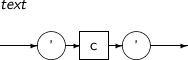
A string literal represents strings. A string literal is enclosed with single quotes (' ') to distinguish it from other schema objects.
A string literal has the following characteristics:
-
The literal can be declared with a size of up to 4,000 bytes.
-
When a string literal is used in an expression or conditional expression, it is handled as a CHAR type.
-
When a string literal is compared with CHAR type data, blank spaces are inserted after the data that has the shorter length before the comparison if the length is different.
-
When a string literal is compared with VARCHAR type data, they are compared without inserting any blank space.
A detailed description of a string literal follows:
-
Syntax
-
Component
Component Description c Characters included in a user character set. ’ To use the escape character in a string literal, single quotes must be added before the first character and after the last character of the literal.
To use single quotes in a string literal,
use the single quote mark two times consecutively.
-
Example
The following example illustrates the use of string literals:
'Tibero' 'Database'
            '2009/11/11'
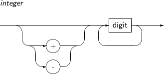
A numeric literal represents integers and real numbers.
The numeric literal has the following characteristics:
-
There are integer and real number literals.
-
When a NUMBER type value exceeds the maximum precision (38 digits), part of the literal is discarded from the end to stay within the precision. If an input literal exceeds the scope that the NUMBER type can specify, an error will occur.
-
Floating point literals are shown below.
Literal Description BINARY_FLOAT_NAN Single-precision NaN (Not A Number) BINARY_FLOAT_INFINITY Single-precision infinity BINARY_DOUBLE_NAN Double-precision NaN (Not A Number) BINARY_DOUBLE_INFINITY Single-precision infinity
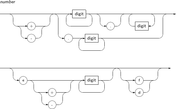
A detailed description of a numeric literal follows:
-
Syntax
-
Component
Component Description digit A number between 0 and 9. + / - A positive/negative sign symbol. . A decimal point. -
Component
Component Description digit A number between 0 and 9. + / - A positive/negative sign symbol.. . A decimal point. e, E For example, 8.33e-4 and 8.33e+4 represent 0.000833 and 83,300 respectively.
"E" can be used instead of "e". Numbers after "e" or "E" are exponential numbers. The exponential number should be between -130 and 125.
f, F BINARY_FLOAT type. A 32-bit floating-point number. d, D BINARY_DOUBLE type. A 64-bit floating-point number. -
Example
The following example illustrates the use of numeric literals:
123 +1.23 0.123
          123e-123 -123
The following example illustrates the use of floating-point literals.
123f +1.23F 0.123d
          -123D
The datetime literal specifies date and time information. DATE, TIME, TIMESTAMP, and TIMESTAMP WITH TIME ZONE literals are classified as datetime literals.
DATE
The DATE literal specifies date and time information.
The DATE literal has the following characteristics:
-
Attributes
The DATE literal has the attributes of century, year, month, day, hour, minute, and second.
-
Literal conversion
By using the TO_DATE function in Tibero, a date value specified with a string or numeric literal can be converted to a DATE literal as well as a particular date can be specified. When a date is specified as a literal, the Gregorian calendar is used.
TO_DATE('2005/01/01
            12:38:20', 'YY/MM/DD HH24:MI:SS')
The default format is 'YYYY/MM/DD' and is defined by the NLS_DATE_FORMAT parameter in an initialization parameter file. The NLS_DATE_FORMAT parameter specifies a date format.
To specify a date value that has no hour information as a DATE literal, the default time will be midnight (HH24 represents 00:00:00 and HH 12:00:00.). To specify a date value that has no date information as a DATE literal, the default date will be the first day of the current month set on the system.
To compare two DATE literals, check that the literals include time information. If only one literal has time information and the other does not, the information must be removed with the TRUNC function before the comparison.
The following example illustrates the use of the TRUNC function:
TO_DATE('2005/01/01', 'YY/MM/DD') = TRUNC(TO_DATE('2005/01/01 12:38:20', 'YY/MM/DD HH24:MI:SS')) -
DATE '2005-01-01'-
There is no time information.
-
The default format is 'YYYY-MM-DD'.
-
In addition to a hyphen, there are several delimiters: slash (/), asterisk (*), period (.), etc.
-
TIME
A TIME literal specifies time information.
The TIME literal has the following characteristics:
-
Attributes
The TIME literal has the attributes of hour, minute, second, and fractional second.
-
Literal conversion
By using the TO_TIME function in Tibero, a time value specified by a string or numeric literal can be converted to a TIME literal, or a particular time can be specified.
TO_TIME('12:38:20.123456789',
            'HH24:MI:SSXFF')
The default format is defined by the NLS_TIME_FORMAT parameter in the initialization parameter file.
-
TIME '10:23:10.123456789' TIME '10:23:10' TIME '10:23' TIME '10'-
The default format is 'HH24:MI:SS.FF9'.
-
Only the hour information in a value cannot be omitted.
-
TIMESTAMP
The TIMESTAMP literal is an expanded version of the DATE literal.
The TIMESTAMP literal has the following characteristics:
-
Attributes
The TIMESTAMP literal has the attributes of year, month, day, hour, minute, second, and fractional second.
-
Literal conversion
By using the TO_TIMESTAMP function in Tibero, a date value specified by a string or numeric literal can be converted to a TIMESTAMP literal.
TO_TIMESTAMP('09-Aug-01
            12:07:15.50', 'DD-Mon-RR HH24:MI:SS.FF')
The default format is defined by the NLS_TIMESTAMP_FORMAT parameter in the initialization parameter file.
-
TIMESTAMP '2005/01/31 08:13:50.112' TIMESTAMP '2005/01/31 08:13:50' TIMESTAMP '2005/01/31 08:13' TIMESTAMP '2005/01/31 08' TIMESTAMP '2005/01/31'-
The default format is 'YYYY/MM/DD HH24:MI:SSxFF'.
-
Date information ('YYYY/MM/DD') in a value cannot be omitted.
-
Fractional second ('FF') can be specified down to the ninth decimal place.
-
TIMESTAMP WITH TIME ZONE
The TIMESTAMP WITH TIME ZONE literal is an expanded version of the TIMESTAMP literal.
The TIMESTAMP WITH TIME ZONE literal has the following characteristics:
-
Attribute
Like the TIMESTAMP literal, the TIMESTAMP WITH TIME ZONE literal has the attributes of year, month, day, hour, minute, second, and fractional second.
-
Literal conversion
By using TO_TIMESTAMP_TZ function in Tiberoa date value specified by a string or numeric literal can be converted to a TIMESTAMP WITH TIME ZONE literal.
TO_TIMESTAMP_TZ('2004-05-15
            19:25:43 Asia/Seoul', 'YYYY-MM-DD HH24:MI:SS.FF TZR')
            TO_TIMESTAMP_TZ('1988-11-21 10:31:58.754 -07:30', 'YYYY-MM-DD
            HH24:MI:SS.FF TZH: TZM')
The default format is defined with the NLS_TIMESTAMP_TZ_FORMAT parameter in the initialization parameter file. The NLS_TIMESTAMP_TZ_FORMAT parameter specifies the format of TIMESTAMP WITH TIME ZONE.
-
TIMESTAMP '1993/12/11 13:37:43.27 Asia/Seoul' TIMESTAMP '1993/12/11 13:37:43.27 +09:00' TIMESTAMP '1993/12/11 13:37:43.27 +07'-
The default format is 'YYYY/MM/DD HH24:MI:SSXFF TZR'.
-
Fractional second ('FF') can be specified down to the ninth decimal place.
-
A time zone('TZR') can be specified with a local name or an offset.
-
If time zone('TZR') is omitted, the value is treated as a TIMESTAMP type literal.
-
TIMESTAMP WITH LOCAL TIME ZONE
The TIMESTAMP WITH LOCAL TIME ZONE literal has the same format as that of the TIMESTAMP literal.
An interval literal specifies the interval between two points in time. An interval can be specified with two formats: a combination of year and month, or with the date, hour, minute, and second.
The interval literal is provided in Tibero with two types:
-
YEAR TO MONTH
Specifies an interval to the nearest month.
-
DAY TO SECOND
Specifies an interval to the nearest minute.
Each type consists of the first field, which is mandatory, and the second field, which is optional. The first field represents a default unit of date or time to be expressed, and the second field represents the smallest interval of the default unit. Interval of the same type can be added to and subtracted from each other.
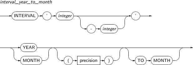
YEAR TO MONTH
The YEAR TO MONTH type specifies a time interval with a year and a month.
A detailed description of the YEAR TO MONTH type follows:
-
Syntax
-
Component
Component Description integer[-integer] A mandatory first field and a second optional field.
The first field is either a year or a month. If the first field represents a year, the second field can be specified and represents a month. The second field must be between 0 and 11.
precision The maximum precision of the YEAR unit.
The value should be an integer between 0 and 9. The default value is 2.
-
Example
The following example illustrates the use of YEAR TO MONTH literals:
INTERVAL '12-3'
          YEAR TO MONTH INTERVAL '123' YEAR(3) INTERVAL '123' MONTH INTERVAL
          '1' YEAR INTERVAL '1234' MONTH(3)
DAY TO SECOND
The DAY TO SECOND type specifies a time interval with a date, an hour, a minute, and a second.
A detailed description of the DAY TO SECOND type follows:
-
Syntax
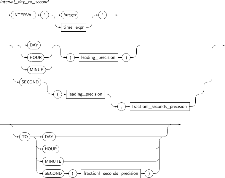
-
Component
Component Description integer The number of days. time_expr Specified with a format such as HH[:MI[:SS[.n]]], MI[:SS[.n]], or SS[.n].
The "n" is the number of digits to the right of the decimal point. If "n" has a larger number of digits than the value set in fractional_seconds_precision, it will be rounded to meet the value in fractional_seconds_precision.
If the first field is DAY, time_expr comes after an integer and one or more blank spaces. The integer indicates the number of days.
leading_precision The precision of the first field.
The value should be an integer between 0 and 9. The default value is 2.
fractional_seconds_precision The precision of the second field.
The value should be an integer between 1 and 9. The default value is 6.
The unit of the first field must be greater than that of the second field. If the second field is HOUR, MINUTE, or SECOND, the value should be between 0 and 23, between 0 and 59, or between 0 and 59.999999999, respectively.
-
Example
The following example illustrates the use of DAY TO SECOND literals:
INTERVAL '1
            2:3:4.567' DAY TO SECOND(3) INTERVAL '1 2:3' DAY TO MINUTE
            INTERVAL '123 4' DAY(3) TO HOUR INTERVAL '123' DAY(3) INTERVAL
            '12:34:56.1234567' HOUR TO SECOND(7) INTERVAL '12:34' HOUR TO
            MINUTE INTERVAL '12' HOUR INTERVAL '12:34' MINUTE TO SECOND
            INTERVAL '12' MINUTE INTERVAL '12.345678'
            SECOND(2,6)
Format strings are used to convert NUMBER and datetime type values to string type values.
Format strings are also used to convert string type values converted from NUMBER type or datetime type values back to their original format values.
String type values can be converted to the NUMBER type or datetime type values, and vice versa. However, the conversion may be impossible depending on the value. For example, the string '12345' can be converted to a NUMBER type value, but the string 'ABCDE' cannot.
Strings that do not follow the default time format or include a non-number character cannot be converted to NUMBER or datetime type values. In this case, transform functions such as TO_DATE and TO_NUMBER are used.
Format strings are used as parameters for the TO_CHAR, TO_DATE, and TO_NUMBER functions. If a parameter is not a format string, the parameter is converted to a format string with a default format.
Note
For more information about TO_CHAR, TO_DATE, and TO_NUMBER functions, refer to “Chapter 4. Functions”.
NUMBER type format strings can be used as parameters for the TO_CHAR and TO_NUMBER functions.
| Function | Description |
|---|---|
| TO_CHAR | Converts a NUMBER type value to a string. |
| TO_NUMBER | Converts a string to a NUMBER type value. |
NUMBER type format strings have the following characteristics:
-
There are various format elements.
The number of digits to the right and left of the decimal point, negative and positive signs, a comma, and an exponent can be output.
-
A symbol that represents a currency unit, such as $ or W, can be inserted.
-
Hexadecimal can be output.
-
A separate string cannot be inserted.
-
There is no format element for distinguishing capital letters from small letters.
The following table shows format elements which may be included in NUMBER type format strings:
| Format Element | Example | Description |
|---|---|---|
| , (comma) | 9,999 | Outputs a comma. A format string cannot start with a comma. |
| . (decimal point) | 99.99 | Outputs a decimal point. A format string can only have a single decimal point. |
| $ | $9999 | Outputs a dollar sign ($) before a number. |
| 0 | 0999 9990 | Adds a 0 before or after a number. It is guaranteed that a 0 will be output if possible. |
| 9 | 9999 | Outputs the number plus an additional character to represent sign. For a positive number, a blank space is output. For a negative number, a minus sign (-) is output. An initial zero will not be output. However, it will output a single zero for the integer 0. |
| B | B9999 | Outputs blanks for zeros. |
| D | 99D99 | Outputs a decimal point. This is the same as the decimal point format element (.). |
| EEEE | 9.9EEEE | Outputs a number in scientific notation. |
| G | 9G999 | Outputs a comma. This is the same as the comma format element (,). |
| L or U | L9999 U9999 | Outputs a dollar symbol before a number. These format elements are the same as the dollar sign format element ($). |
| MI | 9999MI | Outputs a negative sign for a negative number blank space for a positive number. This format element can only be used at the end of a format string. |
| RN (rn) | RN rn | Outputs a Roman numeral. "RN" outputs a numeral with capital letters and "rn" outputs lowercase letters. The numeral can be an integer between 1 and 3,999. |
| S | S9999 9999S | Outputs a positive or negative sign. This element can only be used at the beginning or end of a format string. |
| TM | TM | Expresses a number using the fewest characters possible. "TM9" and "TMe" can also be used. "TM9" is the same as "TM". - "TM9" outputs a fixed point number. - "TMe" outputs a number in scientific notation. - "TM" cannot be used with other format strings. |
The following table shows how a NUMBER type value is output according to each NUMBER format string when the TO_NUMBER function is used.
| NUMBER Type Value | Format String | Output |
|---|---|---|
| 0 | 99.99 | ' .00' |
| 0.1 | 99.99 | ' .10' |
| -0.1 | 99.99 | ' -.10' |
| 0 | 90.99 | ' 0.00' |
| 0.1 | 90.99 | ' 0.10' |
| -0.1 | 90.99 | ' -0.10' |
| 0 | 9999 | ' 0' |
| 1 | 9999 | ' 1' |
| 0.1 | 9999 | ' 0' |
| -0.1 | 9999 | ' -0' |
| 123.456 | 999.999 | ' 123.456' |
| -123.456 | 999.999 | '-123.456' |
| 123.456 | FM999.999 | '123.456' |
| 123.45 | 999.009 | ' 123.450' |
| 123.45 | FM999.009 | '123.45' |
| 123 | FM999.009 | '123.00' |
| 12345 | 99999S | '12345+' |
Datetime type format strings can be used as parameters for the TO_CHAR, TO_DATE, TO_TIMESTAMP, and TO_TIMESTAMP_TZ functions.
| Function | Description |
|---|---|
| TO_CHAR | Converts a datetime type value to a string. |
| TO_DATE | Converts a string to a DATE type value. |
| TO_TIMESTAMP | Converts a string to a TIMESTAMP type value. |
| TO_TIMESTAMP_TZ | Converts a string to a TIMESTAMP_TZ type value. |
Datetime type format strings have the following characteristics:
-
There are various format elements. Output formats for datetime type values such as year, month, day, hour, minute, and second, can be specified.
For example, 'the format element strings 'YYYY' and 'YY', which output a year, output either the last four or last two digits of a year. For example, for the year 2009, '2009' and '09' will be output, respectively.
-
A hyphen (-) or a slash (/) can be inserted. To insert a string that isn't a format element, use double quotes (" ").
-
There are format elements for distinguishing capital letters from lowercase letters. For example, 'DAY', a format element string for outputting a day of the week, outputs all characters with capital letters, 'Day' outputs only the first character with a capital letter, and 'day' outputs all characters with small letters. In the case of Monday, 'MONDAY', 'Monday', and 'monday' will be outputted, respectively.
The following are the format elements that can be used in datetime type.
| Format Element | Argument of TO_* function? | Description |
|---|---|---|
- , . ; : / "text" | - | Outputs the symbol at the corresponding point of the resulting output. |
AD A.D. BC B.C. | Yes | Outputs the value for Anno Domini (A.D.) or for Before Christ (B.C.). |
AM A.M. PM P.M. | Yes | Outputs a value indicating before or after noon. |
CC SCC | No | Outputs a century. (For 2005, 21 is output) SCC adds a minus sign (-) for B.C. |
| D | No | Outputs the number of a day in a week (1-7). |
| DAY | No | Outputs a day of the week (e.g. THURSDAY). |
| DD | Yes | Outputs the number of a day in a month (1-31). |
| DDD | Yes | Outputs the number of a day in a year (1-366). |
| DY | No | Outputs an abbreviated day of the week (e.g. THU). |
| FF[1~9] | Yes | Outputs fractions of a second. The number after the FF is the number of digits to the right of the decimal point to be output. If the number is not specified, it follows the default precision of a data type. |
| FM | No | Format modifier for trimming spaces from the left and right sides before outputting. |
| FX | Yes | Format modifier for determining if the input string is identical to the format string. |
HH HH12 | Yes | Outputs an hour (1-12). |
| HH24 | Yes | Outputs an hour (0-23). |
IYYYY IYYY IYY IY | No | Outputs a 4, 3, 2, or 1 digit year, respectively, following the ISO standard. |
| MI | Yes | Outputs a minute (0-59). |
| MM | Yes | Outputs a month (1-12). |
| MON | Yes | Outputs an abbreviated month (e.g. DEC). |
| MONTH | Yes | Outputs a month (e.g. DECEMBER). |
| Q | No | Outputs a quarter (1-4). |
| RM | Yes | Outputs a month as a roman numeral (I-XII). |
| RR | Yes | Automatically adjusts a century according to an input value of a two-digit year. |
| RRRR | Yes | Outputs a rounded year. A year can be entered using two or four digits. If two digits are entered, this is the same as RR. |
| SS | Yes | Outputs a second (0-59). |
| SSSSS | Yes | Outputs the number of seconds since midnight (0-86,399). |
| WW | No | Outputs the number of a week in a year (1-53). The first week begins on Jan 1, and ends on Jan 7. |
| W | No | Outputs the number of a week in a month (1-5). The first week begins on the first day of the month, and ends on the 7th of the month. |
| X | Yes | Outputs a period (.). |
YEAR SYEAR | No | Outputs a year with words. In the case of SYEAR, a minus sign (-) will be added to a year if it is Before Christ (B.C.). |
YYYY SYYYY | No | Outputs a four-digit year. In the case of SYYYY, a minus sign (-) will be added to a year if it is Before Christ (B.C.). |
YYY YY Y | Yes | Outputs a 3, 2, or 1 digit year, respectively. |
TZH | Yes | Outputs an hour in the time zone. |
TZM | Yes | Outputs a minute in the time zone. |
TZR | Yes | Outputs a region in the time zone. |
TZD | Yes | Outputs an abbreviation of daylight-saving time in the time zone. This value should correspond to the region in TZR. |
| EE | Yes | Outputs Japanese Imperial and Thai Buddha calendars. |
| E | Yes | Outputs an abbreviation of Japanese Imperial and Thai Buddha calendars. |
In the above table, the RR format element is similar to the YY format element but can specify and store a year from another century more easily.
The rules for the RR format element follows:
-
If the last two digits of the current year are between 00 to 49,
-
If a specified two-digit year is between 00 and 49,
The first two digits of the returned year are the same as those of the current year.
-
If a specified two-digit year is between 50 to 99,
The first two digits of the returned year are the same as the current year's first two digits minus one.
-
The following is an example of the RR element for a year between 2000 and 2049:
SQL> SELECT
              TO_CHAR(TO_DATE('20/08/13', 'RR/MM/DD'), 'YYYY') YEAR FROM DUAL;
              YEAR ---------------------------- 2020 SQL> SELECT
              TO_CHAR(TO_DATE('98/12/25', 'RR/MM/DD'), 'YYYY') YEAR FROM DUAL;
              YEAR ---------------------------- 1998
-
-
If the last two digits of the current year are between 50 and 99,
-
If a specified two-digit year is between 00 to 49,
The first two digits of the returned year are the same as the current year's first two digits plus one.
-
If a specified two-digit year is between 50 to 99,
The first two digits of the returned year are the same as those of the current year.
-
The following is an example of the RR element for a year between 1950 and 1999:
SQL> SELECT
              TO_CHAR(TO_DATE('12/10/27', 'RR/MM/DD'), 'YYYY') YEAR FROM DUAL;
              YEAR ---------------------------- 2012 SQL> SELECT
              TO_CHAR(TO_DATE('92/02/08', 'RR/MM/DD'), 'YYYY') YEAR FROM DUAL;
              YEAR ---------------------------- 1992
-
Datetime type format elements can have the following suffixes.
| Suffix | Meaning | Format String | Output Example |
|---|---|---|---|
| TH | An ordinal number | DDTH | 05TH |
| SP | A spelled-out number | DDSP | FIVE |
| SPTH or THSP | An spelled-out ordinal number | DDSPTH | FIFTH |
Note
These suffixes can only be used with a format element that can output a number and only when a number is output.
A format modifier can be specified several times in a format string. Whenever a format modifier is used, it can activate disabled features or inactivate enabled features.
The fill mode (FM) format modifier can change the method for adding spaces, and the format exact (FX) format modifier determines if the input string is identical to the format string.
FM
Tibero adds blank spaces to strings output by a format element to make the length of all the strings identical to the longest string. For example, because the longest string is 'SEPTEMBER' in the MONTH format element, other strings that are months are padded with blank spaces to make their lengths equal to nine characters to match September.
If FM is specified, the method for filling blank spaces is changed to the following:
-
If FM is used for a DATE type format string for the TO_CHAR function,
-
All whitespace characters and zeros added before a character are removed. For example, if April is entered as MM, "4" is output instead of "04".
-
If FM is inactive, all output string lengths for each format element will be the same, but if FM is active, the length of strings may vary depending on the input values.
-
-
If FM is used for a NUMBER type format string for the TO_CHAR function,
-
All whitespace characters before a number and any zeros after a number which were created by the 9 format element are removed. The result will be left-aligned.
-
If FM is inactive, blank characters fill the left side of a number. Therefore, the output will be always right-aligned.
-
FX
Tibero examines if input strings are identical to the format strings. If any string is not the same an error will occur.
If FM is specified, the following restrictions apply:
-
The position of a delimiter or a double quote in the input string should be identical to that in the format string.
-
Additional blank characters are not allowed. If FX is inactive, blank characters are ignored.
-
The number of digits of a number in the input string should be identical to that of each element of the format string.
A pseudo column is automatically inserted into all tables by Tibero without being declared by the user.
The ROWID is an identifier that refers to a row in the entire database. A ROWID contains the physical location of a row, and this value is not changed unless the row is removed.
Tibero uses a multilevel disk structure for storing databases. To search a particular row on a disk using a ROWID, it needs to reflect the disk structure of the ROWID.
ROWIDs in Tibero have the same structure as [Figure 2.1].
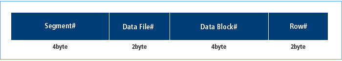
ROWID consists of 12 bytes, including a segment, data file, data block, and row number which are 4, 2, 4, and 2 bytes respectively.
The BASE64 encoding is used for expressing a ROWID value. The encoding expresses a 6-bit number with an 8-bit character by replacing a number between 0 and 63 by A through Z, a through z, 0 through 9, a plus sign (+), or slash (/).
If ROWID is encoded in BASE64, a segment# (6 bytes), data file# (3 bytes), data block# (6 bytes), and row# (3 bytes) are represented in "SSSSSSFFFBBBBBBRRR" format. For example, when a segment#, data file#, data block#, row# are 100, 20, 250, and 0 respectively, the ROWID is "AAAABkAAUAAAAD6AAA".
The ROWNUM is the number of a row when a set of rows is created as a result of a SELECT statement. The first row returned as a result of a query has a value of 1, the second row has 2, the third row has 3, etc.
The following is the method for assigning a ROWNUM in Tibero:
-
A query is executed.
-
Rows are created as a result.
-
Before returning the rows, a ROWNUM is assigned to each row.
Tibero has a ROWNUM counter and assigns the counter value to each row.
-
A conditional expression is applied to the ROWNUM assigned to the row.
-
If the conditional expression is satisfied, the assigned ROWNUM is fixed, and the ROWNUM counter value is incremented by 1.
-
If the conditional expression is not satisfied, the row is discarded, and the ROWNUM counter value is not changed.
ROWNUM can be used to restrict the number of result rows. The following example restricts the returned rows to 10:
SELECT * FROM EMP
      WHERE ROWNUM <= 10;
As a ROWNUM value is assigned near the end of processing a query, even the same SELECT statement can have different results depending on the internal steps of processing the query. For example, a decision by the query optimizer of whether to use an index may have a different result.
The ORDER BY clause can be used to get same results from any query that includes the ROWNUM. However, all subqueries including the WHERE clause are executed, and then the ORDER BY clause is executed in Tibero. Therefore, the ORDER BY clause can also bring different results.
For example, the following query gets different results every time it is executed:
SELECT * FROM EMP
      WHERE ROWNUM <= 10 ORDER BY EMPNO;
If the above query is changed to the following, the results are always identical because the ORDER BY clause is executed first:
SELECT * FROM
      (SELECT * FROM EMP ORDER BY EMPNO) WHERE ROWNUM <=
      10;
The following SELECT statement returns no rows:
SELECT * FROM EMP
      WHERE ROWNUM > 1;
The reason the above statement returns no rows is that the conditional expression for ROWNUM is executed before the ROWNUM value is fixed. The conditional expression is not satisfied because the ROWNUM of the first row is 1, therefore the first row is not returned. Since the conditional expression is not satisfied, the value of the ROWNUM counter is not incremented. Therefore, the ROWNUM of the second row is also 1 and the second row will not be returned. In the end, no results are returned.
LEVEL is the column type for outputting hierarchies of each row in a tree after executing a hierarchical query. The LEVEL value of the top row is 1, and this value is increased by one for each lower row. Output of hierarchical queries and LEVEL column values are described in “5.5. Hierarchical Queries”.
The CONNECT_BY_ISLEAF pseudo column returns "1" if a current row is a leaf of a tree defined by the CONNECT BY condition or "0" if it is not. This information determines whether the row can be extended to show its hierarchy.
The following example illustrates the use of the CONNECT_BY_ISLEAF pseudo column.
SQL> SELECT
      ENAME, CONNECT_BY_ISLEAF, LEVEL, SYS_CONNECT_BY_PATH(ENAME,'-') "PATH"
      FROM EMP2 START WITH ENAME = 'Clark' CONNECT BY PRIOR EMPNO = MGRNO
      ORDER BY ENAME; ENAME CONNECT_BY_ISLEAF LEVEL PATH ---------------
      ----------------- ---------- ----------------------- Alicia 1 3
      -Clark-Martin-Alicia Allen 1 3 -Clark-Ramesh-Allen Clark 0 1 -Clark
      James 1 3 -Clark-Martin-James John 0 3 -Clark-Ramesh-John Martin 0 2
      -Clark-Martin Ramesh 0 2 -Clark-Ramesh Ward 1 4 -Clark-Ramesh-John-Ward
The CONNECT_BY_ISCYCLE pseudo column is used in a hierarchical query. It determines if the row has a child node, and also if the child node can become a parent node of the row. After determining whether or not a loop between the parent node and its child node is possible, the column returns "1" if the row has such a child node or "0" if it does not.
This pseudo column can be used only when a NOCYCLE statement is specified in the CONNECT BY condition. If the NOCYCLE statement is specified, an error will not occur even when a loop occurs.
The following example illustrates the use of the CONNECT_BY_ISCYCLE pseudo column.
SQL> SELECT
      ENAME, CONNECT_BY_ISCYCLE, LEVEL FROM EMP START WITH ENAME = 'Alice'
      CONNECT BY NOCYCLE PRIOR EMPNO = MGRNO ORDER BY ENAME; ENAME
      CONNECT_BY_ISCYCLE LEVEL --------------- ------------------ ----------
      Alice 0 1 Smith 1 2 Micheal 0 3 Viki 0 2 Jane 1 2 Jacob 0 4
When a column in a row has no value, the column is called NULL, or it is said that the column has the NULL value. NULL can be included in a column of any data types which are not restricted by the NOT NULL or PRIMARY KEY constraints. NULL can be used when an actual value is unknown or when a meaningless value is needed. Because NULL is different from 0, NULL should not be expressed with 0. If a column of the string type includes an empty string, it will be treated as NULL.
The result of an arithmetic operation including NULL is always NULL. The result of any operation that includes a NULL, except for an operation including the string concatenation operation (||), is always NULL.
NULL + 1 =
    NULL
If an argument of any constant function except for REPLACE, NVL, and CONCAT is NULL, the return value is also NULL. If the NVL function is used, a non-NULL value can be returned. If a column value is NULL, 0 will be returned, and if the value is non-NULL, the column value will be returned. Most aggregate functions ignore NULL.
The following example illustrates the use of the AVG function with data including NULL:
DATA = {1000, 500,
      NULL, NULL, 1500} AVG(DATA) = (1000 + 500 + 1500) /3 = 1000
There are two comparison conditions, IS NULL and IS NOT NULL, which can check NULL. Because NULL means that there is no data, NULL cannot be compared with NULL or other values. However, two NULLs can be compared with the DECODE function.
SQL> SELECT
      DECODE(NULL, NULL, 1) FROM DUAL; DECODE(NULL,NULL,1) -------------------
      1
In the above example, NULL is compared with NULL using the DECODE function. The result is 1, which means the two values are the same.
If other comparison conditions are used for NULL, the result will be UNKNOWN. In the most cases, UNKNOWN is handled as FALSE. For example, if a WHERE clause in a SELECT statement has a condition judged as UNKNOWN, no row is returned. In the case of UNKNOWN and FALSE, although another operator is used with the UNKNOWN condition, the result will be always UNKNOWN.
The following shows the difference between results of using the NOT operator for FALSE and for UNKNOWN.
NOT FALES = TRUE NOT
      UNKNOWN = UNKNOWN
Comments can be added to SQL statements and schema objects. As comments in a book or a document are used to explain words and sentences, comments in an SQL statement can be used to explain statements.
The contents of a comment can use any characters that can be expressed with the character set used in a database. A comment can be added anywhere between reserve words, parameters, commas, etc. Comments do not influence the execution of an SQL statement.
Comments allow users to read and manage application source code easily. For example, SQL statements that have comments regarding their usage and purpose can be more easily understood.
There are two ways to add a comment:
-
Use a comment start delimiter (/*) and a comment end delimiter (*/).
This kind of comment can span multiple lines. Comments do not need to use a blank space or a carriage return to separate the start delimiter (/*) and end delimiter (*/) from the comment itself.
-
Use the comment delimiter (--).
This kind of comment cannot span multiple lines. It uses the carriage return to determine the end of the comment.
The following example illustrates the use of comments in SQL statements:
SELECT emp_id,
    emp_name, e.dept_id /* Outputs a list of employees in the general affairs
    department. */ /* Table */ FROM emp e, dept d WHERE e.dept_id = d.dept_id
    AND d.dept_name = 'The General Affairs Department' AND e.status != 1; /*
    Excludes resigned people. */ SELECT emp_id, emp_name, e.dept -- Outputs a
    list of employees in -- the material dept. -- Table FROM emp e, dept d
    WHERE e.dept_id = d.dept_id AND d.dept_name = 'Materials Department' AND
    e.status != 1; -- Excludes resigned people.
It is also possible to add comments to schema objects as well as SQL statements. Comments can be added to schema objects such as tables, views, and columns using the COMMENT syntax. Comments added in a schema object are saved in a data dictionary.
A hint is a kind of directive. Using a hint, a particular action can be sent to Tibero's query optimizer or the query optimizer's execution plan can be changed. The query optimizer cannot always make an optimized execution plan. Developers can modify the execution plan of the query optimizer directly using hints.
An SQL statement block can include only one hint. The hint must be located immediately after a SELECT, UPDATE, INSERT, or DELETE statement.
The following examples illustrate the use of hints:
(DELETE|INSERT|SELECT|UPDATE)
      /*+ hint [hint] ... */
or
(DELETE|INSERT|SELECT|UPDATE)
    --+ hint [hint] ...
When using a hint, note the following:
-
A hint can only be located after a SELECT, UPDATE, INSERT, or DELETE statement.
-
A plus sign (+) must be located immediately after a comment delimiter ('/*' or '--') without any space.
-
A space between the hint and the plus sign (+) is allowed.
-
A syntactically incorrect hint is treated as a comment and does not raise an error.
A detailed description of various hints follows:
| Type | Hint | Description |
|---|---|---|
| Query transformation | NO_QUERY_ TRANSFORMATION | Instructs the query transformer to not change the entire queries. |
| NO_MERGE | Instructs the query transformer to not merge views for specific views. | |
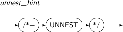
| UNNEST | Instructs the query transformer to unnest specific subqueries. | |
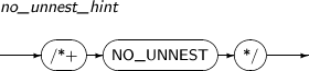
| NO_UNNEST | Instructs the query transformer not to unnest specific subqueries. | |
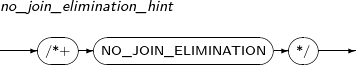
| NO_JOIN_ELIMINATION | Instructs the query transformer not to eliminate joins. | |
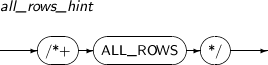
| Optimizer mode | ALL_ROWS | Instructs the query optimizer to optimize the method for the handling process to maximize result throughput. |
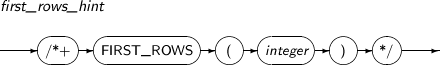
| FIRST_ROWS | Instructs the query optimizer to optimize the method for an output result with the fastest response. | |
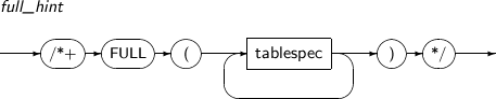
Access mode | FULL | Instructs the query optimizer to perform a full table scan. |
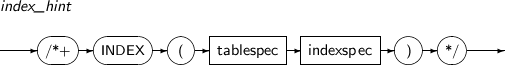
| INDEX | Instructs the query optimizer to perform an index scan using a specified index. | |
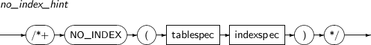
| NO_INDEX | Instructs the query optimizer not to perform an index scan using a specified index. | |
| INDEX_ASC | Instructs the query optimizer to perform an index scan using a specified index in ascending order. | |
| INDEX_DESC | Instructs the query optimizer to perform an index scan using a specified index in descending order. | |
| INDEX_FFS | Instructs the query optimizer to perform a fast full index scan using a specified index. | |
| NO_INDEX_FFS | Instructs the query optimizer not to perform a fast full index scan using a specified index. | |
| INDEX_RS | Instructs the query optimizer to perform a range index scan using a specified index. | |
| NO_INDEX_RS | Instructs the query optimizer not to perform a range index scan using a specified index. | |
| INDEX_SS | Instructs the query optimizer to perform an index skip scan using a specified index. | |
| NO_INDEX_SS | Instructs the query optimizer to not perform an index skip scan using a specified index. | |
| INDEX_JOIN | Instructs the table to self join using two or more indexes. | |
| Join order | LEADING | Instructs the query optimizer to use a specified set of tables that must be joined first. |
| ORDERED | Instructs the query optimizer to join tables in the order specified in the FROM clause. | |
| Join mode | USE_NL | Instructs the query optimizer to use a nested loop join. |
| NO_USE_NL | Instructs the query optimizer not to use a nested loop join. | |
| USE_NL_WITH_INDEX | Instructs the query optimizer to use a nested loop join using a specified index and join conditions. | |
| USE_MERGE | Instructs the query optimizer to use a merge join. | |
| NO_USE_MERGE | Instructs the query optimizer not to use a merge join. | |
| USE_HASH | Instructs the query optimizer to use a hash join. | |
| NO_USE_HASH | Instructs the query optimizer not to use a hash join. | |
| HASH_SJ | Instructs the query optimizer to use hash semi-join when unnesting a subquery. | |
| HASH_AJ | Instructs the query optimizer to use hash anti-join when unnesting a subquery. | |
| MERGE_SJ | Instructs the query optimizer to use merge semi-join when unnesting a subquery. | |
| MERGE_AJ | Instructs the query optimizer to use merge anti-join when unnesting a subquery. | |
| NL_SJ | Instructs the query optimizer to use nested loop semi-join when unnesting a subquery. | |
| NL_AJ | Instructs the query optimizer to use nested loop anti-join when unnesting a subquery. | |
| SWAP_JOIN_INPUTS | Instructs the query optimizer to build tables when performing a hash join. | |
| NO_SWAP_JOIN_INPUTS | Instructs the query optimizer not to change the join order when performing a hash join. | |
| Parallel processing | PARALLEL | Instructs the query optimizer to use a specified number of threads to execute queries in parallel. |
| NO_PARALLEL | Instructs the query optimizer not to execute queries in parallel. | |
| PQ_DISTRIBUTE | Instructs the query optimizer to specify the distribution mode for rows for parallel joins. | |
| Materialized view | REWRITE | Instructs the query optimizer to rewrite queries using a materialized view without cost comparison. |
| NO_REWRITE | Instructs the query optimizer not to rewrite queries.. | |
| Others | APPEND | Instructs the query optimizer to execute the Direct-Path method, which writes directly to a data file in DML statements. |
| APPEND_VALUES | Instructs the query optimizer to execute the Direct-Path method, which writes directly to a data file in INSERT statement with the VALUES clause. | |
| NOAPPEND | Instructs the query optimizer not to execute the Direct-Path method in DML statements. | |
| IGNORE_ROW_ON_ DUPKEY_INDEX | Instructs the optimizer not to generate an error when a row that violates unique constraint is inserted. | |
| CARD | Instructs the optimizer to use a given value to calculate a specified table's cardinality when optimizing a query. | |
| MONITOR | Instructs the optimizer to collect query execution information. | |
| NO_MONITOR | Instructs the optimizer to not collect query execution information. | |
| USE_CONCAT | Instructs the optimizer to create OR expansion plans. | |
| NO_EXPAND | Instructs the optimizer not to perform OR expansion. |
Hints about query transformations influence the query transformation method of Tibero. Only the NO_MERGE hint can currently be used.
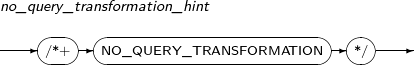
NO_QUERY_TRANSFORMATION
Instructs the query transformer to avoid all query changes. Tibero automatically performs query transformation and creates an execution plan for the optimized query. If the NO_QUERY_TRANSFORMATION hint is used, query transformation, which is enabled by default, is not performed.
-
Syntax
NO_MERGE
Instructs the query transformer not to merge specific views. Views are merged by default in Tibero. The merged view forms a single query block by combining with an upper query block. However, the NO_MERGE hint prevents views from being merged.
-
Syntax
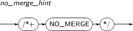
-
Example
The following example illustrates the use of the NO_MERGE hint:
SELECT * FROM
          T1, (SELECT /*+ NO_MERGE */ * FROM T2, T3 WHERE T2.A = T3.B) V WHERE
          T1.C = V.D
As shown above, the NO_MERGE hint is specified in a query block of a view that must not be merged. If there is no hint, views will be merged, and the optimizer will consider the join order and method for the tables T1, T2, and T3. However, if there is a hint as in the above example, T2 and T3 are joined first and then T1 is joined later.
UNNEST
Instructs the query transformer to unnest specific subqueries. Subqueries are unnested by default in Tibero . To unnest only a specific query, disable the unnesting function with the initialization parameter and use the UNNEST hint by specifying it in the desired subquery block.
-
Syntax
NO_UNNEST
Instructs the query transformer not to unnest specific subqueries. Subqueries are unnested by default in Tibero. If subqueries can be unnested, the subqueries will be transformed by joining. At this time, the NO_UNNEST hint prevents subqueries from being unnested. This hint is specified in a subquery block.
-
Syntax
NO_JOIN_ELIMINATION
Instructs the query transformer not to eliminate unnecessary joins. Joins that are needed to generate query results are eliminated by default in Tibero . This can be prevented by using the NO_JOIN_ELIMINATION hint.
-
Syntax
-
Example
The following is an example of using the NO_JOIN_ELIMINATION hint.
SELECT /*+
          NO_JOIN_ELIMINATION */ T2.FK, T2.A FROM T1, T2 WHERE T2.FK =
          T1.PK
In the previous example, if a relationship is defined between T1 and T2 and a column from T2 is requested, the two tables are linked with the condition T2.FK = T1.PK without explicitly joining them as long as T2.FK is not null. Such elimination by the query optimizer can be prevented by using the NO_JOIN_ELIMINATION hint.
The handling process and result output can be optimized using optimizer mode hints. If a query uses an optimizer mode hint, the query will be handled as if it has no statistics information or values for the optimizer mode for initialization parameters.
ALL_ROWS
Instructs the optimizer to optimize the method for the handling process to maximize result throughput with minimum resources.
-
Syntax
FIRST_ROWS
Instructs the query optimizer to optimize the method to provide the fastest response for the output result for the first n rows, where n is provided via a parameter.
-
Syntax
Hints about access modes instructs the query optimizer to use a specific access mode if possible. If the mode is not possible to use, the optimizer ignores the hint.
The table name specified in the hint must be the same as the one used in the SQL statement. If an alias is used for a table, the table alias must be used instead of the table name. Even if a table name in an SQL statement includes a schema name, only the table name is necessary in the hint.
FULL
Instructs the query optimizer to perform a full table scan when a given table is scanned. Even if there is an index which meets the conditional expression specified in a WHERE clause, a full table scan is executed.
-
Syntax
INDEX
Instructs the query optimizer to perform an index scan using a specified index when a given table is scanned.
-
Syntax
NO_INDEX
Instructs the optimizer not to perform an index scan when a given table is scanned. If NO_INDEX and INDEX, INDEX_ASC, or INDEX_DESC specify the same index, the query optimizer ignores both hints.
-
Syntax
INDEX_ASC
Instructs the query optimizer to perform an index scan using a specified index when a given table is scanned. If an index scan is used, the index is scanned in ascending order. As the default order for index scans in Tibero is already by ascending order, INDEX_ASC returns the same result as INDEX. In the case of a partitioned index, each partition is scanned in ascending order.
-
Syntax

INDEX_DESC
Instructs the query optimizer to perform an index scan using a specified index when a given table is scanned. If an index scan is used, the index is scanned in descending order. In the case of a partitioned index, each partition is scanned in descending order.
-
Syntax
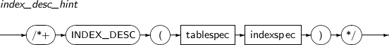
INDEX_FFS
Instructs the query optimizer to perform a fast full index scan using a specified index for a specified table.
-
Syntax

NO_INDEX_FFS
Instructs the query optimizer not to perform a fast full index scan using a specified index for a specified table.
-
Syntax
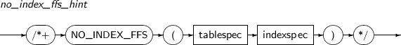
INDEX_RS
Instructs the query optimizer to perform a range index scan using a specified index.
-
Syntax

NO_INDEX_RS
Instructs the query optimizer not to perform a range index scan using a specified index.
-
Syntax
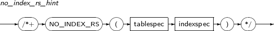
INDEX_SS
Instructs the query optimizer to perform an index skip scan using a specified index.
-
Syntax
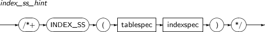
NO_INDEX_SS
Instructs the query optimizer not to perform an index skip scan using a specified index.
-
Syntax
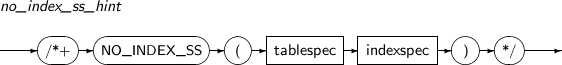
INDEX_JOIN
Instructs the table to self join using two or more indexes when scanning the table.
-
Syntax
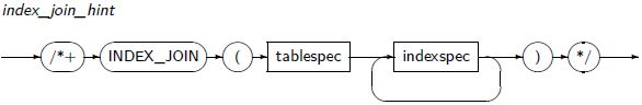
Hints about join order, LEADING and ORDERED, determine the join order. Because the LEADING hint gives more options to the query optimizer than the ORDERED hint does, using the LEADING hint rather than the ORDERED hint is recommended.
LEADING
Instructs the query optimizer to use a specified set of tables that must be joined first. If the LEADING hint includes a table that cannot be joined first, the hint is ignored. If two or more LEADING hints conflict, all LEADING and ORDERED hints are ignored. If the ORDERED hint is used, all LEADING hints are ignored.
-
Syntax
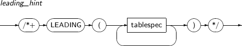
ORDERED
Instructs the query optimizer to join tables in the order specified in a FROM clause. The query optimizer has information about the size of a result set of joins. It is recommended to use this hint only when a user clearly understands the join order from information provided by the query optimizer.
-
Syntax
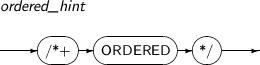
Hints about the join mode change the mode for joining a table. These hints are only available when the specified table is used as the inner table for joining. If the specified table is used as an outer table, the hints are ignored.
USE_NL
Instructs the query optimizer to use a nested loop join when a specified table is joined with other tables.
-
Syntax
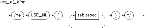
NO_USE_NL
Instructs the query optimizer not to use a nested loop join when a specified table is joined with other tables. However, in certain circumstances, the query optimizer can still create a plan that uses nested loop joins.
-
Syntax

USE_NL_WITH_INDEX
Instructs the query optimizer to use a nested loop join when a specified table is joined with other tables. The specified table should be accessed using a specified index and join conditions for the two tables. If the index cannot be used, the hint is ignored.
-
Syntax
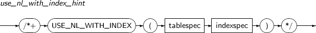
USE_MERGE
Instructs the query optimizer to use a merge join when a specified table is joined with other tables.
-
Syntax
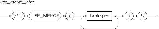
NO_USE_MERGE
Instructs the query optimizer not to use a merge join when a specified table is joined with other tables.
-
Syntax
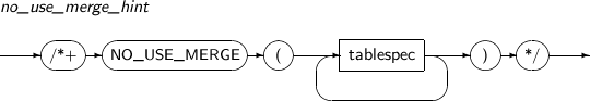
USE_HASH
Instructs the query optimizer to use a hash join when a specified table is joined with other tables.
-
Syntax
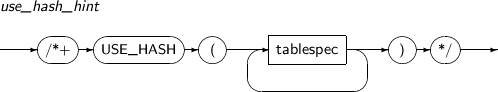
NO_USE_HASH
Instructs the query optimizer not to use a hash join when the specified table is joined with other tables.
-
Syntax
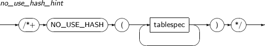
HASH_SJ
Instructs semi-join using hash when unnesting a subquery.
-
Syntax
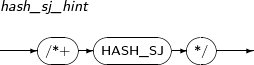
HASH_AJ
Instructs anti-join using hash when unnesting a subquery.
-
Syntax
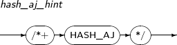
MERGE_SJ
Instructs the query optimizer to use merge semi-join when unnesting a subquery.
-
Syntax

MERGE_AJ
Instructs the query optimizer to use merge anti-join when unnesting a subquery.
-
Syntax
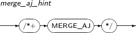
NL_SJ
Instructs the query optimizer to use nested loop semi-join when unnesting a subquery.
-
Syntax
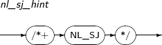
NL_AJ
Instructs the query optimizer to use nested loop anti-join when unnesting a subquery.
-
Syntax

SWAP_JOIN_INPUTS
Instructs the query optimizer to build tables when performing a hash join.
-
Syntax
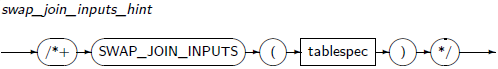
NO_SWAP_JOIN_INPUTS
Instructs the query optimizer not to change the join order when performing a hash join.
-
Syntax
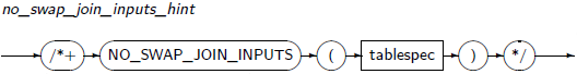
PARALLEL
Instructs the query optimizer to use a specified number of threads to execute queries in parallel.
-
Syntax
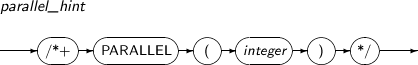
NO_PARALLEL
Instructs the query optimizer not to execute queries in parallel.
-
Syntax
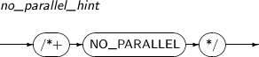
PQ_DISTRIBUTE
Instructs the query optimizer to use a specific distribution method for rows to be joined during parallel processing of queries. The methods are HASH-HASH, BROADCAST-NONE, NONE-BROADCAST, and NONE-NONE. Selecting a specific distribution method can enhance the performance of a join during parallel processing.
-
Syntax
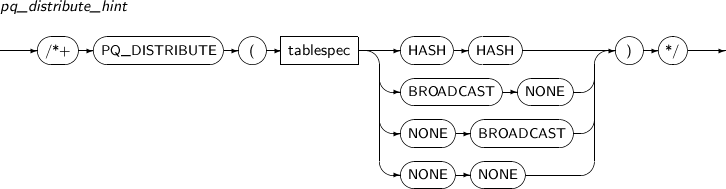
The following describes each property.
Property Description NONE NONE Generates a plan as if there is no hint. BROADCAST NONE Acts like a combination of a left join 'BROADCAST' and a right join ' PE BLOCK ITERATOR'. NONE BROADCAST Acts like a combination of a left join 'PE BLOCK ITERATOR' and a right join ' BROADCAST'. HASH HASH Acts like a combination of the left and right hash joins.
REWRITE
Instructs the query optimizer to rewrite a query using a materialized view in the query block without comparing costs. The optimizer compares the result of rewriting the query block with the REWRITE hint with the result of rewriting all blocks and selects the better option. When a list of materialized views is specified, a query rewrite is only attempted on the materialized views in the list.
-
Syntax
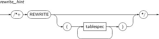
NO_REWRITE
Instructs the query optimizer not to rewrite a query in the query block.
-
Syntax
APPEND
Instructs the query optimizer to execute the Direct-Path method, which writes directly to a data file in DML statements. Unlike other insert methods, Direct-Path inserts data with newly allocated data blocks and directly inserts data files without using the buffer cache, which enhances batch performance.
-
Syntax
APPEND_VALUES
Instructs the query optimizer to execute the Direct-Path method, which writes directly to a data file in INSERT statement with the VALUES clause. Unlike other insert methods, Direct-Path inserts data with newly allocated data blocks and directly inserts data files without using the buffer cache, which enhances batch performance.
-
Syntax
NOAPPEND
Instructs the query optimizer not to execute the Direct-Path method in DML statements.
-
Syntax
IGNORE_ROW_ON_DUPKEY_INDEX
Only available for single table insert statements. If an insert violates a unique constraint, the row is rolled back and an insert is performed starting in the next row without generating an error. An error is generated when an index is not defined, multiple indexes are defined, or a defined index does not have unique property. If a hint is defined, the APPEND and PARALLEL hints are ignored.
-
Syntax
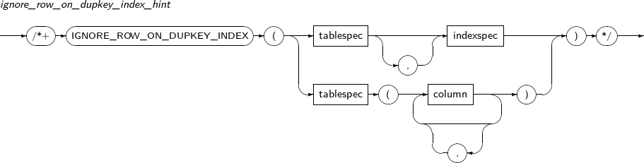
CARD
Instructs the optimizer to use a given value to calculate a specified table's cardinality when optimizing a query.
-
Syntax
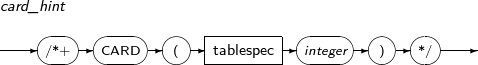
MONITOR
Instructs the optimizer to collect query execution information.
-
Syntax
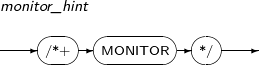
NO_MONITOR
Instructs the optimizer not to collect query execution information.
-
Syntax
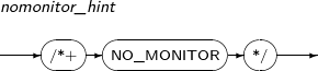
USE_CONCAT
Forces to create an OR expansion plan by concatenating combined OR conditions in a clause to a compound query with UNION ALL.
-
Syntax
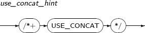
NO_EXPAND
Forces to create a plan with an OR condition by preventing the optimizer from performing OR expansion.
-
Syntax
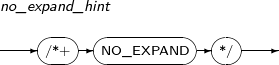
A database consists of many objects. Every object is part of the following inclusion relationship: 'Database > User > Schema > Schema Object'. A database is shared by several users. Among the users, there is a database administrator (DBA) who has the authority to manage the database.
A schema is a collection of objects that belong to users. A user can define only one schema and the schema name is the same as the user name in Tibero.
A Schema Object is an object included in a schema. Apart from the schema objects defined in the SQL standard, additional schema objects are provided depending on the database.
Tibero provides the following schema objects:
-
Table
-
Index
-
View
-
Sequence
-
Synonym
A Table is the basic storage unit of a relational database. All other schema objects are defined with tables as the basic unit. A table has the form of a two-level matrix. A table consists of one or more columns, and each column has its own data type. A table includes zero or more rows, and each row has a value for each column.
Note
To create, modify, or delete a table, use the CREATE TABLE, ALTER TABLE, or DROP TABLE SQL statement, respectively. These statements are part of the data definition language (DDL). For more information about DDL, refer to “Chapter 7. Data Definition Language”.
The following example shows a table that has information about employees:
[Example 2.1] EMP Table
 EMPNO ENAME ADDR
        SALARY DEPTNO ---------- ------------ ---------------- ----------
        ---------- 35 John Houston 30000 5 54 Alicia Castle 25000 4 27 Ramesh
        Humble 38000 5 69 James Houston 35000 4
The above table consists of five columns (EMPNO, ENAME, ADDR, SALARY, and DEPTNO) and four rows. Column information that defines a table is rarely changed, but the number of rows included in a table can be changed at any time.
For some column data types, like the string type, the maximum length needs to be set, and for some column types, like the NUMBER type, precision and scale need to be set. A default value can be set for some columns. For more information about data types, refer to “2.1. Data Types”.
Integrity constraints can be declared for an entire table or for individual columns. All rows inserted in a table must satisfy the integrity constraints. For example, the following constraint can be declared for the column SALARY in the table EMP:
SALARY >=
      0
As a salary of an employee cannot be less than 0, the above condition prevents incorrect data from being entered. Conditional expressions to declare integrity constraints are described in “3.4. Conditional Expressions”.
An integrity constraint can be declared for one table, and a referential integrity constraint can be declared between two tables.
The following example shows the DEPT table that contains information about departments:
[Example 2.2] DEPT Table
 DEPTNO DNAME LOC
        ---------- ------------ ---------------- 1 Accounting Houston 4
        Research Spring 5 Sales Houston
If each employee must be a member of a particular department, the values of the column DEPTNO in the table EMP in [Example 2.1] must match one of the values of the column DEPTNO in the table DEPT in [Example 2.2].
Note
For more information about integrity constraints, refer to Tibero Administrator's Guide.
An index is the data structure that enables searching a particular column in a table rapidly by using a separate storage space from the table. A table owner can create one or more indexes for a particular column.
Note
To create, modify, or delete an index, use the CREATE INDEX, ALTER INDEX, or DROP INDEX SQL statement respectively. These statements are included in the data definition language (DDL). For more information, refer to “Chapter 7. Data Definition Language”.
Descriptions of indexes are as follows:
-
Automatic indexing
In Tibero indexes are automatically created for the primary key columns in a table. A primary key column has a value that uniquely identifies a particular row in a table. Two different rows in a table cannot have the same value in a primary key column. In the above examples, [Example 2.1] and [Example 2.2], EMPNO and DEPTNO could be the primary key column respectively.
-
Allowance for duplicate values of columns
An index can be created regardless of column values. For example, an index can be created for the column DEPTNO, which has duplicate values in the table EMP. An index can also be created for the column DEPTNO, which has no duplicate values in the table DEPT.
-
Allowance for multiple columns
An index can be created for more than one column by joining the values of two or more columns. For example, an index can be created for the columns ENAME and ADDR by joining the values of the two columns. This kind of index is useful when more than one column is searched simultaneously.
-
Application of indexes
After an index is created by a user, the index is not automatically used. When executing an SQL query the query optimizer compares the execution efficiency of using an index with the efficiency of not using the index. The query is executed in the more efficient way.
The database system automatically decides whether to use the table index or the index for a specific column.
-
Management of indexes
Indexes are automatically managed by the database system. Whenever a row is inserted, updated, or deleted in a table, all indexes in the table are updated.
-
Deletion of indexes
An index can be deleted if the index is no longer needed. Extra indexes may hinder performance because indexes are updated whenever a modification occurs in a table. Removing unnecessary indexes is recommended.
The purpose of a view is to represent frequently executed queries in a way that is similar to a table. A view is defined using a table or another view and can be used like a general table within a SQL statement. The table where views are defined is called a base table.
As a table can be accessed by multiple users, views can be defined to secure information by hiding some parts of the table information from particular users.
Note
To create or delete a view, use the CREATE VIEW or DROP VIEW SQL statement respectively. These statements are included in the data definition language (DDL). For more information, refer to “Chapter 7. Data Definition Language”.
Descriptions of views follow:
-
View merging
Views manage query statements as a kind of string in a database system. When a SQL statement including views is entered, the database system transforms the statement to an SQL statement for the base table that does not include the views. This process is called view merging.
-
Using views and the authorizations
Views can be used to show only a part of a base table as well as to simplify frequently used queries. For example, if the value of the column SALARY in the table EMP must not be accessed by employees outside of the managerial department, a view can be created that allows general employees to access the table EMP through the view instead of accessing the table EMP directly.
This example is related to the authority to access schema objects. If the user who defines a view grants the authority to general employees to access the view but does not grant the authority to access the table EMP, the employees can only search the part of the table that is in the view.
A sequence is a schema object that generates unique sequential values. The value is generally used for a primary key or a unique key. In a sequence name, a pseudo column name is always attached.
SQL statements read the sequence value through the following pseudo columns:
| Column | Description |
|---|---|
| CURRVAL | Returns NEXTVAL that is queried lastly in the current session. |
| NEXTVAL | Increases the current value of the sequence and returns the increased value. |
The following example illustrates the use of a sequence with pseudo columns:
seq1.currval
      seq2.nextval
The following describes the availability of sequence pseudo columns according to the location in an SQL statement:
| Availability | Location |
|---|---|
| Available |
(except a SELECT list of subqueries or views)
|
| Unavailable |
|
When a sequence is created, its initial value, incremental value, and decremental value are defined. When a sequence is accessed for the first time through the pseudo column NEXTVAL, the sequence returns the initial value. Whenever NEXTVAL is used, the value of the sequence is increased by the incremental value and the newly increased value is returned. The pseudo column CURRVAL always returns the current value of the sequence, and this value is the same as the value returned by the last use of NEXTVAL.
To use the pseudo column CURRVAL, initialize this column using NEXTVAL at least one time. When the pseudo column NEXTVAL is used in a SQL statement, it increases the sequence value by the number of rows handled by the SQL statement.
Rows which increase sequence values are:
-
A row output by a top-level SELECT statement
-
A row selected by the SELECT statement in an INSERT ... SELECT statement
-
A row selected by the SELECT statement in a CREATE TABLE ... AS SELECT statement
-
A row updated by an UPDATE statement
-
A row inserted by an INSERT statement that includes a VALUES statement
If more than one NEXTVAL appears in the same row, the sequence value is increased only once in the first location, and the value will be used in the following locations.
If NEXTVAL and CURRVAL appear in the same row, the sequence value is increased once, and the value returned by NEXTVAL will be used in CURRVAL.
A synonym is an alias defined for a particular schema object. A synonym is usually defined for a schema object which has a particular purpose or has a long name.
Note
To create or delete a synonym, use the SQL statement CREATE SYNONYM or DROP SYNONYM respectively. These statements are included in the data definition language (DDL). There is no SQL statement for modifying a synonym. For more information, refer to “Chapter 7. Data Definition Language”.
Descriptions of synonyms follow:
-
Difference between a synonym and a view
Both synonyms and views are used to replace longer names. However, a synonym is only used for one schema object while a view is for a complete SQL statement. Access authority for a synonym is not configured separately, unlike a view. If a user has access authority for a particular schema object, the user also has access authority for the synonym of the schema object.
-
Configuring a synonym
A synonym can be used only by the user who defined the synonym, or it can be defined to be shared by all users. A synonym that can be shared by all users is called a shared synonym. In Tibero various system views and synonyms for each view are defined so that DBAs and general users can easily access the data dictionary information.
A user has to give a name to each schema object or to the whole schema objects by the objects such as table, table column, index, integrity constraint, table partition, table subpartition, index partition, index subpartition, package, and functions and procedures in the package.
To specify the name of a schema object in SQL, use an identifier with double quotes or an identifier without double quotes.
-
An identifier with double quotes starts and ends with a double quote (").
-
An identifier without double quotes does not use the double quotes.
Any identifier can be used to name a schema object. An identifier with double quotes is case sensitive while an identifier without double quotes is not case sensitive and treats all letters as capital letters.
For example, the following are all different identifiers:
department
      "department" "Department"
The following are all the same identifier:
department
      DEPARTMENT "DEPARTMENT"
Identifiers must comply with the following rules:
-
The length must not exceed 30 bytes.
-
Reserved words cannot be used as an identifier without double quotes. Reserved words can be used as an identifier by using quotation marks, but this is not recommended. Refer to “Appendix A. Reserved Words” for more information about reserved words.
-
An identifier without double quotes can have only alphabetic letters, Korean letters, numbers, underscores (_), dollar signs ($), and hashes (#). However, numbers, dollar signs ($), and hashes (#) cannot be the first character.
-
An identifier with double quotes may use any letter or symbol, including blank spaces. However, double quotes (" ") themselves cannot be used as part of the identifier.
-
Two different objects in the same namespace cannot have the same name.
Classification Namespace Type Schema object General object Tables, views, materialized views, sequences, synonyms, and packages. Functions and procedures that are not included in the package. Independent namespace
Indexes and triggers.
(Namespaces in different schemas are not shared. Therefore, two tables in different schemas can have the same name.)
General object Independent namespace User roles, shared synonyms, and tablespaces. -
Two different columns in a table cannot have the same name. Columns in different tables can have the same name.
-
Any two procedures or functions in a package can have the same name if they have a different number of parameters or have different data types.
This section describes how to specify a schema object and components of the object using SQL statements.
Detailed descriptions of the syntax that specifies schema objects follow:
-
Syntax
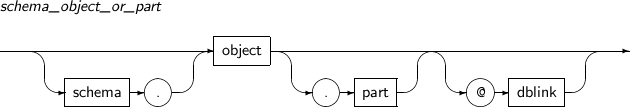
-
Component
Component Description schema The name of a schema that includes an object.
By specifying the schema component, an object in a different user's schema can be specified. To access the object, access authority is required. If this part is omitted, an object in the local schema is specified.
The qualifier "schema" can be used only for a schema object. For information about schema types, general objects and namespace, refer to “2.9.6. Schema Object Names”.
The qualifier "PUBLIC" is used for shared synonyms. For this qualifier, double quotes (" ") must be used.
object The name of an object. part Used to specify components of an object. For example, the components of a table are columns, partitions , etc. dblink Used for distributed database functions. Specify the database name that contains the object specified in the component object.
dblink is used to specify an object in remote database instead of local database. If this qualifier is omitted, it is considered that an object in user database is specified.
How to search for a schema object
The process to search for a schema object specified in an SQL statement is as follows:
-
Determine the namespace based on the SQL statement.
-
Search for the object within the determined namespace.
-
Determine if the specified type can be used for the purpose described by the SQL statement.
-
If the type cannot be used, return an error.
The following illustrates the above process:
SELECT *
      FROM employees;
The above SQL statement is entered. The following numbers represent each step of the above search process.
-
The SQL statement does not specify a schema, so the user's schema becomes the namespace.
-
Search for an object named employees within the determined namespace (in this case, the user's schema). If there is no such object, check if there is a shared synonym called "employees". If there is not, return an error.
If the found object is a synonym, check if the schema object defined by the synonym is also a synonym. If the defined object is also a synonym, check if the next defined object is also a synonym. Repeat this process until a non-synonym schema object results.
-
Check if the object is a table or a view because only these objects may be used in a FROM statement.
-
If the object is not a table or a view, return an error.
How to search an object in a remote database
To specify an object in a remote database, specify the object name with the at symbol (@) and a database link. A database link is a schema object that enables access to a remote database. For more information about how to create a database link, refer to “7.25. CREATE DATABASE LINK”.
The process to search for an object when a database link is used in a SQL statement is as follows:
-
Search for the database link in the user's schema.
-
If there is no database link, search shared database links.
-
If a database link is found, try to access the database object using the link..
-
The process to search for a schema object in a remote database is the same as described above in How to search a schema object.